Understanding PageRank Algorithm - How Google's PageRank Actually Works

Introduction

PageRank is the algorithm that put Google on the map literally and figuratively. Developed by Larry Page and Sergey Brin at Stanford, PageRank revolutionized web search by treating links as votes of confidence. A page linked by many important pages is itself important. This recursive definition creates an elegant mathematical problem: computing the stationary distribution of a random walk on the web graph.

In this tutorial, I'll walk you through implementing PageRank from scratch, exploring what happens when the algorithm encounters dead-end nodes, and understanding why real-world implementations need damping factors. We'll use the power iteration method to compute PageRank scores and visualize convergence behavior.

The PageRank Concept

Imagine a random web surfer clicking links indefinitely. PageRank measures the probability of finding this surfer on any given page after many clicks. Pages with more incoming links from important pages accumulate higher probabilities.

The key insight: link structure reveals importance. A page linked by The New York Times homepage carries more weight than a page linked by my personal blog. PageRank captures this transitivity of importance.

Building the Transition Matrix

The first step is converting a graph of web pages and links into a transition matrix where each column represents the probability of moving from one page to another.

import pandas as pd
import numpy as np

def create_transition_matrix(edges, nodes):
    '''
    Create transition matrix from edge list using pandas DataFrame.
    edges: list of tuples (from_node, to_node)
    nodes: list of node names
    '''
    # Create adjacency matrix as DataFrame
    adj_matrix = pd.DataFrame(0, index=nodes, columns=nodes)

    # Fill in the edges by selecting the location in the matrix
    for src, dst in edges:
        adj_matrix.loc[dst, src] += 1

    # Calculate out-degrees
    out_degrees = adj_matrix.sum(axis=0)

    # Create transition matrix by normalizing columns
    transition_matrix = adj_matrix.div(out_degrees, axis=1).fillna(0)

    return transition_matrix

Understanding the Implementation

Adjacency Matrix Construction: I start with a matrix of zeros where rows and columns represent nodes. For each edge from src to dst, I increment adj_matrix[dst, src]. Notice the reversed indexing this is intentional for column-stochastic matrices.

Out-Degree Calculation: Summing column-wise gives the number of outgoing links from each node. A page with 5 outgoing links distributes its PageRank equally among those 5 pages (each gets 1/5).

Normalization: Dividing each column by its sum ensures columns sum to 1, creating a proper probability distribution. The .fillna(0) handles nodes with no outgoing links (we'll see why this is problematic later).

Computing PageRank via Power Iteration

PageRank is the dominant eigenvector of the transition matrix. We can find it using power iteration repeatedly multiplying the matrix by a vector until convergence.

def compute_pagerank(M, iterations=50, tolerance=1e-6):
    '''
    Compute PageRank using power iteration method.
    M: transition matrix (pandas DataFrame)
    iterations: maximum number of iterations
    tolerance: convergence threshold
    '''
    n = M.shape[0]

    # Initialize with uniform distribution
    v = pd.Series(1/n, index=M.index)

    print(f'Initial distribution:\n{v}\n')

    for i in range(iterations):
        # Matrix-vector multiplication
        v_new = M.dot(v)

        # Check convergence
        diff = (v_new - v).abs().sum()

        print(f'Iteration {i+1}:')
        print(f'{v_new}\n')

        if diff < tolerance:
            print(f'Converged after {i+1} iterations')
            break

        v = v_new

    return v

Why Power Iteration Works

The transition matrix has a special property: its largest eigenvalue is 1 (for strongly connected graphs). The corresponding eigenvector is the PageRank distribution. Power iteration amplifies the dominant eigenvector while suppressing others.

Initialization: Starting with uniform distribution (each page gets 1/n probability) ensures we don't bias toward any particular page.

Convergence Check: When the L1 norm of the difference between consecutive iterations falls below our tolerance, we've converged. This typically happens within 20-50 iterations for small graphs.

Example 1: Computing PageRank for a Simple Graph

Let's apply this to a concrete example:

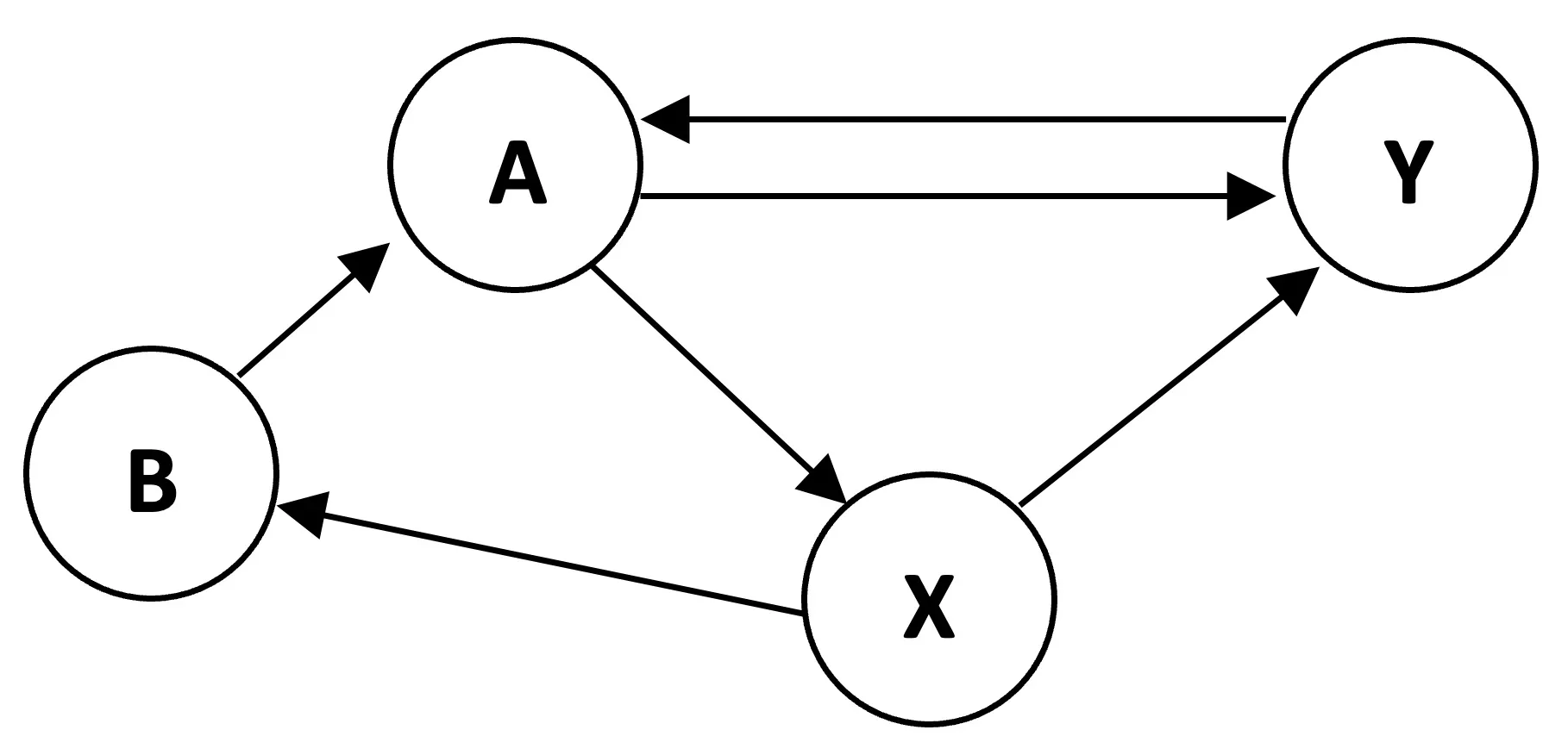
# Define edges based on the graph
edges_a = [
    ('A', 'Y'),
    ('A', 'X'),
    ('B', 'A'),
    ('X', 'B'),
    ('X', 'Y'),
    ('Y', 'A')
]

nodes_a = ['A', 'B', 'X', 'Y']

print('\nEdges:', edges_a)
print('Nodes:', nodes_a)
print()

# Create transition matrix
M_a = create_transition_matrix(edges_a, nodes_a)

print('Transition Matrix M:')
print(f'{M_a}')

Output:

Edges: [('A', 'Y'), ('A', 'X'), ('B', 'A'), ('X', 'B'), ('X', 'Y'), ('Y', 'A')]
Nodes: ['A', 'B', 'X', 'Y']

Transition Matrix M:
     A    B    X    Y
A  0.0  1.0  0.0  1.0
B  0.0  0.0  0.5  0.0
X  0.5  0.0  0.0  0.0
Y  0.5  0.0  0.5  0.0

Interpreting the Transition Matrix

• Column A: Node A has 2 outgoing links (to Y and X), so each gets probability 0.5
• Column B: Node B has 1 outgoing link (to A), so A gets probability 1.0
• Column X: Node X has 2 outgoing links (to B and Y), so each gets probability 0.5
• Column Y: Node Y has 1 outgoing link (to A), so A gets probability 1.0

Now let's compute PageRank:

# Compute PageRank
pagerank_a = compute_pagerank(M_a, iterations=50)

print('FINAL PAGERANK:')
print(f'{pagerank_a}\n')

Convergence Output (abbreviated):

Initial distribution:
A    0.25
B    0.25
X    0.25
Y    0.25
dtype: float64

Iteration 1:
A    0.500
B    0.125
X    0.125
Y    0.250
dtype: float64

Iteration 2:
A    0.3750
B    0.0625
X    0.2500
Y    0.3125
dtype: float64

...

Iteration 10:
A    0.387097
B    0.129032
X    0.193548
Y    0.290323
dtype: float64

Converged after 10 iterations

Understanding the Results

Node A has the highest PageRank (0.387) because it receives links from both B and Y, and Y itself has decent PageRank.

Node Y comes second (0.290) with incoming links from A and X.

Node X (0.194) and Node B (0.129) have lower PageRank because they receive fewer incoming links from important pages.

The algorithm converged in just 10 iterations! The rapid convergence happens because this is a small, well-connected graph.

Example 2: The Dead-End Node Problem

Now let's explore what happens when nodes have no outgoing links dead ends:

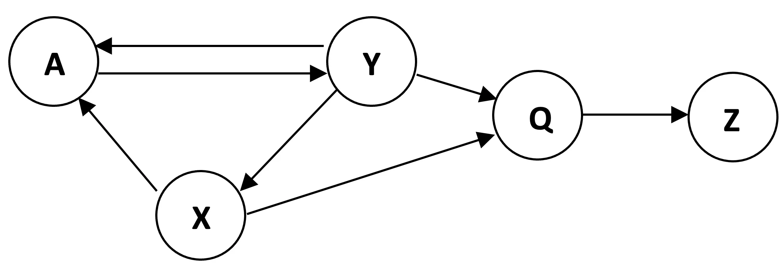
# Define edges for graph with dead-end nodes Q and Z
edges_b = [
    ('A', 'Y'),
    ('A', 'X'),
    ('X', 'Y'),
    ('Y', 'A'),
    ('Y', 'Q'),
    ('Y', 'Z')
]

nodes_b = ['A', 'X', 'Y', 'Q', 'Z']

# Create transition matrix
M_b = create_transition_matrix(edges_b, nodes_b)

print('Transition Matrix M:')
print(f'{M_b}')

Output:

Transition Matrix M:
     A    X    Y    Q    Z
A  0.0  0.0  0.5  0.0  0.0
X  0.5  0.0  0.0  0.0  0.0
Y  0.5  1.0  0.0  0.0  0.0
Q  0.0  0.0  0.25 0.0  0.0
Z  0.0  0.0  0.25 0.0  0.0

Notice that columns Q and Z are all zeros they have no outgoing links. This is a problem.

# Compute PageRank
pagerank_b = compute_pagerank(M_b, iterations=50)

print('FINAL PAGERANK:')
print(f'{pagerank_b}\n')

print(f"PageRank of Q: {pagerank_b['Q']:.6f}")
print(f"PageRank of Z: {pagerank_b['Z']:.6f}")

Convergence Output (abbreviated):

Initial distribution:
A    0.2
X    0.2
Y    0.2
Q    0.2
Z    0.2
dtype: float64

Iteration 1:
A    0.200
X    0.100
Y    0.300
Q    0.050
Z    0.050
dtype: float64

...

Iteration 44:
A    5.099750e-07
X    3.053513e-07
Y    6.834944e-07
Q    5.099750e-07
Z    6.834944e-07
dtype: float64

Converged after 44 iterations

FINAL PAGERANK:
A    6.834944e-07
X    4.092474e-07
Y    9.160540e-07
Q    6.834944e-07
Z    9.160540e-07
dtype: float64

PageRank of Q: 0.000001
PageRank of Z: 0.000001

The Probability Leak Problem

All PageRank scores converge to near-zero! This is the dead-end node problem in action.

Here's what happens:

1. Random surfer starts with uniform probability across all nodes
2. As iterations progress, probability flows through the graph
3. When the surfer reaches Q or Z, they get stuck no outgoing links to follow
4. Probability accumulates in dead ends and never returns to the rest of the graph
5. Over time, all probability "leaks out" of the system into these dead ends
6. Eventually, the entire graph drains to zero

This demonstrates why real PageRank implementations use a damping factor (typically 0.85). The damping factor models a random surfer who occasionally gets bored and jumps to a random page instead of following links. This prevents probability from getting trapped in dead ends.

The modified PageRank formula becomes:

PageRank(p) = (1-d)/N + d * Σ(PageRank(q) / OutDegree(q))

Where d is the damping factor (0.85), N is the total number of pages, and the sum is over all pages q linking to p.

Key Insights

1. Link Structure Encodes Importance

PageRank successfully identifies important nodes based purely on graph topology. In our first example, node A emerged as most important because it received links from other well-connected nodes.

2. Dead Ends Break the Algorithm

Without special handling, dead-end nodes cause probability leakage. This is why production PageRank implementations add:

• Damping factor: Teleportation to random pages
• Dead-end handling: Redistribute stuck probability uniformly

3. Convergence Speed Varies

Small, well-connected graphs converge quickly (10 iterations). Graphs with dead ends take longer (44 iterations) and converge to degenerate solutions.

4. Matrix Operations Are Key

PageRank reduces to linear algebra: finding the dominant eigenvector of a stochastic matrix. This enables efficient computation even for billions of web pages using sparse matrix techniques.

5. Column-Stochastic Matters

The transition matrix must be column-stochastic (columns sum to 1) for proper probability interpretation. This requires careful normalization by out-degrees.

Practical Applications

PageRank extends far beyond web search:

Social Network Analysis: Identify influential users based on follower graphs

Citation Networks: Rank academic papers by citation importance (used by Google Scholar)

Recommendation Systems: Rank products based on co-purchase graphs

Fraud Detection: Identify suspicious accounts in transaction networks

Protein Interaction Networks: Find key proteins in biological systems

When to Use PageRank

Use PageRank when:

• You have a directed graph representing relationships or links
• Importance should be determined by network structure, not just degree
• You want to account for the quality of incoming links, not just quantity
• You need a scalable algorithm (works on graphs with billions of nodes)

Don't use PageRank when:

• Your graph is undirected (use other centrality measures)
• You have explicit importance signals (use supervised learning instead)
• The graph changes rapidly (PageRank requires recomputation)
• You need real-time results (power iteration takes multiple passes)

Conclusion

This project demonstrated how PageRank transforms graph structure into importance scores through elegant linear algebra. By implementing the algorithm from scratch, I gained deep understanding of transition matrices, power iteration, and the critical role of damping factors.

The dead-end node experiment revealed why naive implementations fail probability leaks out of the system, causing all scores to collapse to zero. This explains why Google's original PageRank included the damping factor: it's not just an optimization, it's essential for correctness.

Understanding PageRank deeply not just using a library function enables making informed decisions about graph analysis, centrality measures, and network-based ranking systems. When you see how matrix multiplication propagates importance through a network, when you understand why dead ends break the algorithm, when you know why damping factors matter you become a better data scientist.

The ability to rank nodes by network structure has applications far beyond web search. Any domain with relational data social networks, citation graphs, transaction networks can benefit from PageRank's elegant approach to measuring importance.

📓 Jupyter Notebook

Want to explore the complete code and run it yourself? Access the full Jupyter notebook with detailed implementations and visualizations:

→ View Notebook on GitHub

You can also run it interactively:

• Open in Google Colab
• Open in Binder

🎁 Bonus: Run-Length Encoding for String Compression

As a bonus, let's explore a completely different algorithm: run-length encoding (RLE), a simple yet effective compression technique for strings with repeated characters.

What is Run-Length Encoding?

RLE compresses strings by replacing sequences of identical characters with the character and its count. For example:

• "AAAAABBBBCCCCAA" becomes "A,5;B,4;C,4;A,2"
• "WWWWWWWWWWWWBWWWWWWWWWWWWBBBWWWWWWWWWWWWWWWWWWWWWWWWWB" becomes "W,12;B,1;W,12;B,3;W,24;B,1"

This is particularly effective for data with long runs of repeated values, such as:

• Binary images (long sequences of black or white pixels)
• Fax transmissions
• Simple graphics
• Genomic sequences with repeated nucleotides

Implementation

Here's a clean Python implementation that reads from STDIN and outputs the compressed string:

import sys

def run_length_encoding(input_str: str) -> str:
    result = []
    # store the current character
    cur_char = input_str[0]
    # store the count of the current character
    count = 1

    # loop starts from second character until the end of input string
    for i in range(1, len(input_str)):
        # until the characters found are same as the current character increase count
        if input_str[i] == cur_char:
            count += 1
        # if a new character is found which is not the current character
        # append the character and it's count and change the current character as the new character
        else:
            result.append(f"{cur_char},{count};")
            cur_char = input_str[i]
            count = 1
    # appending the last character and it's count after the loop ends
    result.append(f"{cur_char},{count}")
    return "".join(result)


if __name__ == "__main__":
    # read from STDIN
    input_string = sys.stdin.read().strip()

    # perform run length encoding
    output = run_length_encoding(input_string)
    # print output
    print(output)

How It Works

1. Initialize: Store the first character as cur_char and set count = 1
2. Iterate: Loop through remaining characters
3. Match: If current character equals cur_char, increment count
4. Mismatch: When a different character appears:
   • Append "character,count;" to result
   • Update cur_char to the new character
   • Reset count to 1
5. Finalize: After the loop, append the last character and its count

Running the Script

You can run this script from the command line using STDIN:

echo "AAAAABBBBCCCCAA" | python run_length_encoding.py

Output:

A,5;B,4;C,4;A,2

Compression Analysis

Let's analyze the compression ratio:

Original: "AAAAABBBBCCCCAA" = 15 characters

Compressed: "A,5;B,4;C,4;A,2" = 16 characters

Wait, it got longer! This highlights an important limitation of RLE: it only provides compression when runs are long enough. For short runs, the overhead of encoding (character + comma + count + semicolon) actually increases size.

Break-even point: A run of 3 identical characters:

• Original: "AAA" = 3 characters
• Encoded: "A,3;" = 4 characters (worse)
• Run of 4: "AAAA" = 4 characters vs "A,4;" = 4 characters (same)
• Run of 5: "AAAAA" = 5 characters vs "A,5;" = 4 characters (better!)

For runs of 5+ characters, RLE provides compression. For shorter runs, it's counterproductive.

When to Use RLE

Use RLE when:

• Data has long runs of repeated values (images, fax, simple graphics)
• You need fast, simple compression with minimal CPU overhead
• You want lossless compression
• Data is already somewhat structured (not random)

Don't use RLE when:

• Data is highly random (no repeated runs)
• You need maximum compression (use gzip, bzip2, or modern algorithms)
• Runs are typically short (overhead dominates)
• You're compressing text (use dictionary-based compression instead)

Real-World Applications

Image Compression: Early image formats like PCX and BMP used RLE for simple graphics with large solid-color areas.

Fax Transmission: RLE is part of the CCITT fax compression standard for black-and-white documents.

Video Encoding: Some video codecs use RLE as a component for compressing frame differences.

Data Storage: Databases use RLE for compressing columns with many repeated values.

Conclusion

Run-length encoding demonstrates that simple algorithms can be powerful in the right context. While it won't compress random data or text effectively, it excels at compressing data with long repeated runs. Understanding when and why RLE works (or doesn't) is more valuable than just knowing the algorithm.

The implementation showcases clean Python practices: reading from STDIN, building results incrementally, and handling edge cases (the final character). These patterns apply to many string processing tasks beyond compression.

📄 Python Script

Access the complete run-length encoding implementation:

→ View Script on GitHub