Building a Movie Recommendation System with Apache Spark on AWS EMR

Introduction

Recommendation systems power some of the most successful platforms today—from Netflix suggesting your next binge-worthy series to Amazon recommending products you didn't know you needed. At their core, these systems analyze patterns in user behavior to predict preferences. In this tutorial, I'll walk you through building a movie recommendation system using Apache Spark on AWS EMR, processing 10 million movie ratings to find similar films based on collaborative filtering.

We'll leverage cosine similarity to measure how alike two movies are based on user rating patterns. If many users rate two movies similarly, those movies are likely similar in nature. This approach scales beautifully with Spark's distributed computing model, making it perfect for big data applications.

Part 1: Setting Up AWS Infrastructure

Step 1: Launch EC2 Instance

First, we need an EC2 instance to manage our EMR cluster and access AWS services:

1. Navigate to AWS EC2 console
2. Launch a new instance (t2.micro for free tier is sufficient for management tasks)
3. Configure security groups to allow SSH access
4. Download your key pair for SSH authentication

Step 2: Create S3 Bucket for Data Storage

S3 will serve as our distributed file system for storing the MovieLens dataset:

1. Navigate to AWS S3 console
2. Create a new bucket (e.g., jonesh-test)
3. Keep default settings for versioning and encryption
4. Note the bucket name for later use

Step 3: Upload MovieLens 10M Dataset

Download the MovieLens 10M dataset from GroupLens:

• Dataset size: ~10 million ratings
• Users: ~72,000 users
• Movies: ~10,000 movies
• Files: ratings.dat, movies.dat, tags.dat

Extract the ml-10M100K folder and upload it to your S3 bucket:

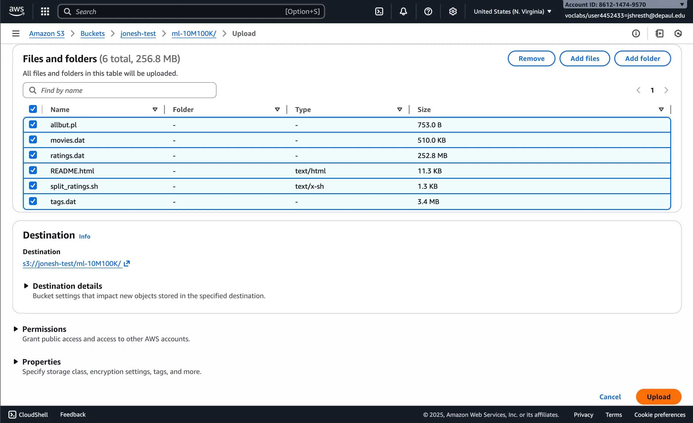
Figure 1: Drag and drop the ml-10M100K folder to upload to S3 bucket

Step 4: Create EMR Cluster

Now we'll create an EMR cluster with Spark installed:

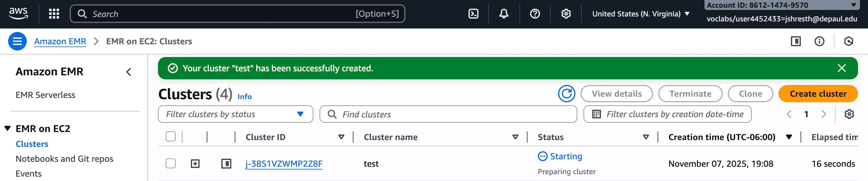
Figure 2: Creating EMR cluster with 3 core instances and 1 master instance

Cluster Configuration:

• Master node: 1 instance (m5.xlarge recommended)
• Core nodes: 3 instances (m5.xlarge recommended)
• Applications: Spark, Hadoop, JupyterHub
• Total nodes: 4 (1 master + 3 core)

Alternatively, if you've created an EMR cluster before, you can clone it:

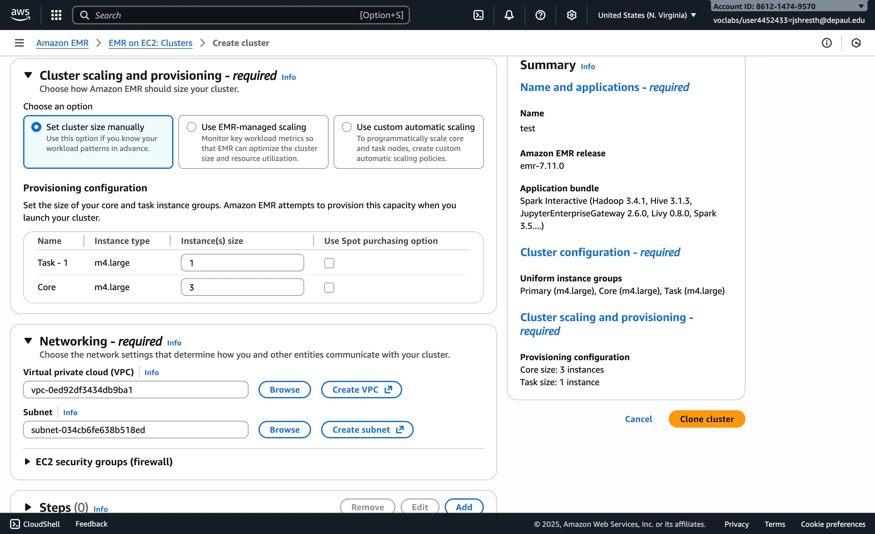
Figure 3: Cloning a previous 4-node EMR cluster configuration

Step 5: Launch JupyterLab from EMR Studio

Once your cluster is running, attach it to EMR Studio to launch JupyterLab:

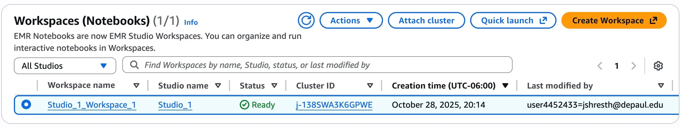
Figure 4: Attaching EMR cluster to Workspaces (Notebooks) to launch JupyterLab

This opens a JupyterLab environment with PySpark pre-configured, allowing you to run distributed Spark jobs interactively.

Part 2: Loading and Exploring the Data

Reading Ratings Data from S3

First, we'll read the ratings.dat file from our S3 bucket into a Spark DataFrame:

# get the ml-10M100K folder path from s3 bucket
path = 's3://jonesh-test/ml-10M100K/'

# read ratings.dat from the s3 bucket location with delimiter '::' to Spark DataFrame with header
# inferSchema is set to true to convert any numerical values into integer/float
ratings = (spark.read
          .option('delimiter', '::')
          .option('inferSchema', 'true')
          .csv(path + 'ratings.dat')
          .toDF('UserID', 'MovieID', 'Rating', 'Timestamp'))

Output:

+------+-------+------+---------+
|UserID|MovieID|Rating|Timestamp|
+------+-------+------+---------+
|     1|    122|   5.0|838985046|
|     1|    185|   5.0|838983525|
|     1|    231|   5.0|838983392|
|     1|    292|   5.0|838983421|
|     1|    316|   5.0|838983392|
+------+-------+------+---------+
only showing top 5 rows

Reading Movies Metadata

Next, we'll load the movie titles and genres:

# read movies.dat from the s3 bucket location with delimiter '::' to Spark DataFrame with header
# inferSchema is set to true to convert any numerical values into integer/float
movies = (spark.read
         .option('delimiter', '::')
         .option('inferSchema', 'true')
         .csv(path + 'movies.dat')
         .toDF('MovieID', 'Title', 'Genres'))

Output:

+-------+--------------------+--------------------+
|MovieID|               Title|              Genres|
+-------+--------------------+--------------------+
|      1|    Toy Story (1995)|Adventure|Animati...|
|      2|      Jumanji (1995)|Adventure|Childre...|
|      3|Grumpier Old Men ...|      Comedy|Romance|
|      4|Waiting to Exhale...|Comedy|Drama|Romance|
|      5|Father of the Bri...|              Comedy|
+-------+--------------------+--------------------+
only showing top 5 rows

Part 3: Computing Movie Similarities

Step 1: Create Movie Pairs

The key insight for collaborative filtering is finding movies that were rated by the same users. We'll perform a self-join on the ratings DataFrame:

# import all necessary functions like col, agg, sqrt, etc. from pyspark
from pyspark.sql.functions import *

# compute movie pairs rated by the same user for cosine similarity computation
# ratings dataframe is joined with itself based on same UserID and 
# r1.MovieID < r2.MovieID to ensure each movie pair appears only once (avoiding duplicates like [1,2] and [2,1])
# then used select to create four columns dataframe with MovieIDs and Ratings named movie_pairs
movie_pairs = ratings.alias('r1').join(ratings.alias('r2'),
                                       (col('r1.UserID') == col('r2.UserID')) &
                                       (col('r1.MovieID') < col('r2.MovieID'))
                                      ).select(col('r1.MovieID').alias('movie1'),
                                               col('r2.MovieID').alias('movie2'),
                                               col('r1.Rating').alias('rating1'),
                                               col('r2.Rating').alias('rating2'))

Output:

+------+------+-------+-------+
|movie1|movie2|rating1|rating2|
+------+------+-------+-------+
|     5|   253|    3.0|    3.0|
|     5|   345|    3.0|    4.0|
|     5|   454|    3.0|    3.0|
|     5|   736|    3.0|    4.0|
|     5|   780|    3.0|    5.0|
+------+------+-------+-------+
only showing top 5 rows

Why r1.MovieID < r2.MovieID?
This condition ensures each movie pair appears only once. Without it, we'd get both (1, 2) and (2, 1), which are redundant for similarity computation.

Step 2: Compute Cosine Similarity Components

Cosine similarity measures the angle between two rating vectors. The formula is:

We'll compute the numerator and denominator components:

# using the movie_pairs to compute components needed for cosine similarity
# first grouped by movie1 and movie2 and count the number of users that rated both movies as numPairs
# then compute sum of element-wise products of the two rating vectors (sum_xy),
# sum of squared ratings for movie1 (sum_xx)
# sum of squared ratings for movie2 (sum_yy)
pair_scores = movie_pairs.groupBy('movie1', 'movie2').agg(
    count('*').alias('numPairs'),
    sum(col('rating1') * col('rating2')).alias('sum_xy'),
    sum(col('rating1') * col('rating1')).alias('sum_xx'),
    sum(col('rating2') * col('rating2')).alias('sum_yy'))

Output:

+------+------+--------+--------+--------+--------+
|movie1|movie2|numPairs|  sum_xy|  sum_xx|  sum_yy|
+------+------+--------+--------+--------+--------+
|     1|  2004|    1772|18875.25|28299.75|14830.75|
|     1|  2668|     588|  6289.5| 10397.5| 4421.25|
|     1|  2994|      33|   444.0|  485.75|  441.75|
|     1|  3809|    2208|29898.25| 36551.0|27035.25|
|     1|  4241|     199|  1160.0|  3125.0|  715.25|
+------+------+--------+--------+--------+--------+
only showing top 5 rows

Step 3: Calculate Final Similarity Scores

Now we'll compute the actual cosine similarity and filter for high-quality recommendations:

# compute cosine similarity
cosine_similarities = pair_scores.withColumn('score', col('sum_xy') / (sqrt(col('sum_xx')) * sqrt(col('sum_yy'))))
# filter the cosine similarities where numPairs >= 10 i.e. only if more than 10 users have rated both movies
# and cosine similarity scores are greater than 0.95 to store only the most similar movie pairs
similarities_filtered = cosine_similarities.filter(col('numPairs') >= 10).filter(col('score') >= 0.95)

Output:

+------+------+--------+--------+--------+---------+------------------+
|movie1|movie2|numPairs|  sum_xy|  sum_xx|   sum_yy|             score|
+------+------+--------+--------+--------+---------+------------------+
|     1|  1208|    6449|102072.0|100414.0|113210.75|0.9573387913508588|
|     1|  1348|    1136|17080.75|17666.25| 18250.25|0.9512624225282171|
|     1|  1357|    2873| 44755.5|47380.25| 45733.25| 0.961461075725028|
|     1|  3304|     109| 1549.25| 1758.75|  1483.75|0.9590452167312737|
|     1|  3668|    1022|14785.75|16644.75|  14431.5|0.9540013377015786|
+------+------+--------+--------+--------+---------+------------------+
only showing top 5 rows

Filtering Rationale:

• numPairs >= 10: Ensures statistical significance (at least 10 users rated both movies)
• score >= 0.95: Only keeps highly similar movies (95%+ similarity)

Part 4: Finding Similar Movies

Get Top 10 Movies Similar to Toy Story

Let's find movies most similar to "Toy Story" (MovieID = 1):

# get top 10 movies most similar to Toy Story (MovieID = 1)
# filter for pairs where movie1 = 1, then order by similarity score descending and limit to 10 results
toy_story_similarities = similarities_filtered.filter(col('movie1') == 1).orderBy(col('score').desc()).limit(10)

Output:

+------+------+--------+------+------+------+------------------+
|movie1|movie2|numPairs|sum_xy|sum_xx|sum_yy|             score|
+------+------+--------+------+------+------+------------------+
|     1| 36553|      10| 143.0|162.75| 126.5|0.9966215554619151|
|     1|  6336|      13| 180.5|207.75| 158.5|0.9946998598171956|
|     1| 41831|      17| 244.0|274.75|219.75|0.9930166580182394|
|     1| 60341|      10|137.25|170.75| 112.0|0.9924827921220798|
|     1|  8422|      17|234.25| 249.5| 223.5|0.9919860408658672|
|     1| 55895|      15| 227.5| 255.0| 207.0|0.9902073326897796|
|     1|  7273|      11| 157.5| 234.5| 108.0|0.9896856126772272|
|     1| 25931|      12|169.25| 217.5| 134.5|0.9895503677685183|
|     1| 32781|      24|332.25|439.75| 256.5| 0.989278067592776|
|     1| 62801|      17|266.75|267.25|272.25|0.9889210628340293|
+------+------+--------+------+------+------+------------------+

Format Results with Movie Titles

Finally, let's join with the movies DataFrame to get human-readable titles:

# formatting for final output
# join the movies dataframe with the toy_story_similarities based on the movieID for both movie1 and movie2
# select the Title from movies based on the join and add columns to top_similar_movies_with_names dataframe and scores
top_similar_movies_with_names = toy_story_similarities.join(
    movies.alias('m1'), toy_story_similarities.movie1 == col('m1.MovieID')).join(
    movies.alias('m2'), toy_story_similarities.movie2 == col('m2.MovieID')).select(
    col('m1.Title').alias('Movie Name'),
    col('m2.Title').alias('Similar Movies'),
    col('score'))
# order by score descending
top_similar_movies_with_names = top_similar_movies_with_names.orderBy(col('score').desc())

Final Output:

+----------------+--------------------+------------------+
|      Movie Name|      Similar Movies|             score|
+----------------+--------------------+------------------+
|Toy Story (1995)|In Old Chicago (1...|0.9966215554619151|
|Toy Story (1995)|Marooned in Iraq ...|0.9946998598171956|
|Toy Story (1995)|They Died with Th...|0.9930166580182394|
|Toy Story (1995)|Standard Operatin...|0.9924827921220798|
|Toy Story (1995)|    Kings Row (1942)|0.9919860408658672|
|Toy Story (1995)|Desperate Hours, ...|0.9902073326897796|
|Toy Story (1995)|Piece of the Acti...|0.9896856126772272|
|Toy Story (1995)|  Road to Rio (1947)|0.9895503677685183|
|Toy Story (1995)|       Hawaii (1966)| 0.989278067592776|
|Toy Story (1995)|Lone Wolf and Cub...|0.9889210628340293|
+----------------+--------------------+------------------+

Key Insights and Observations

1. Distributed Computing Power

Spark's distributed architecture allows us to process 10 million ratings across 4 nodes efficiently. The self-join operation, which would be computationally expensive on a single machine, is parallelized across the cluster.

2. Similarity Threshold Matters

By setting score >= 0.95, we ensure only highly similar movies are recommended. Lower thresholds would return more results but with potentially weaker correlations.

3. Statistical Significance

The numPairs >= 10 filter ensures recommendations are based on sufficient user overlap. Movies rated by only 1-2 common users might show high similarity by chance.

4. Collaborative Filtering Limitations

Notice that "Toy Story" (an animated children's film) shows high similarity to "In Old Chicago" (a 1937 drama). This happens because collaborative filtering finds movies rated similarly by the same users, not necessarily movies with similar content. Users who rate both films highly might have eclectic tastes.

Performance Considerations

Spark Optimization Techniques Used:

1. DataFrame API: More optimized than RDD API with Catalyst optimizer
2. Lazy Evaluation: Spark builds an execution plan before running computations
3. In-Memory Computing: Intermediate results cached in memory across nodes
4. Partitioning: Data automatically distributed across cluster nodes

Scaling Further:

• Increase cluster size: Add more core nodes for larger datasets
• Tune Spark configurations: Adjust executor memory, cores, and partitions
• Use Spark MLlib: Built-in ALS (Alternating Least Squares) for more sophisticated recommendations

Conclusion

We've successfully built a scalable movie recommendation system using Apache Spark on AWS EMR, demonstrating:

• AWS infrastructure setup: EC2, S3, and EMR cluster configuration
• Distributed data processing: PySpark DataFrames for big data operations
• Collaborative filtering: Cosine similarity-based recommendations
• Real-world application: Processing 10 million ratings to find similar movies

This approach scales to billions of ratings and can be adapted for various recommendation scenarios—from e-commerce products to music streaming platforms. The key is leveraging Spark's distributed computing model to handle massive datasets efficiently.

Next Steps:

• Implement content-based filtering for hybrid recommendations
• Add user-based collaborative filtering (find similar users)
• Deploy as a real-time recommendation API using Spark Streaming
• Experiment with matrix factorization techniques (ALS)

📓 Jupyter Notebook

Want to explore the complete code and run it yourself? Access the full Jupyter notebook with detailed implementations:

→ View Notebook on GitHub

You can also run it interactively:

• Open in Google Colab
• Open in Binder

Note: Running this notebook requires AWS EMR cluster access. For local testing, consider using the smaller MovieLens 100K dataset.